Geomagnetism.org

Certain mass extinction events, including the largest ever 250 million years ago, have been argued to have been triggered by the eruption of “large igneous provinces” (LIPs) – humongous plateaux comprising stacks of lava flows that erupted in relatively short amounts of time.

But how short a time? This is a crucial question as the atmosphere and oceans are pretty effective at processing the gases associated with volcanic eruptions in the short to medium term. So, unless the eruptions occur very close together (i.e. just years apart), there is not really much scope for them causing the kind of long term climate change that can wipe out large fractions of life.

Here at Liverpool, we just published a paper outlining a new tool for getting a handle on eruption rates based on the similarity of the magnetic field direction recorded in cooled lava flows that are on top of one another. The logic goes:

– the Earth’s magnetic field is changing direction all the time (which is why you have to change the declination on your compass every few years)

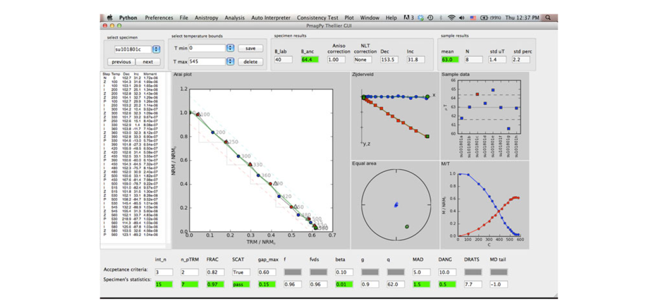
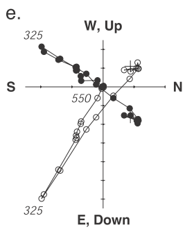
– when magma erupts and then cools, the magnetic minerals in the newly formed rock lock in a record of this direction

– if neighbouring lavas erupted within a few years of one another then the magnetic field direction will not have changed very much so the directions recorded in them will be quite similar.

This is not a new idea but the paper presents and tests a new parameter for formally quantifying the degree of this “next neighbour correlation”. The new parameter was shown to be an improvement over existing methods and its application to lavas from the  60 million year old “North Atlantic LIP” gave some quite surprising results. There was already independent evidence showing, that in one section of this large igneous province, there were pauses between eruptions that were, on average, several tens of thousands of years  long. Unexpectedly, significant similarity was observed in magnetic directions measured in neighbouring lavas from this section.

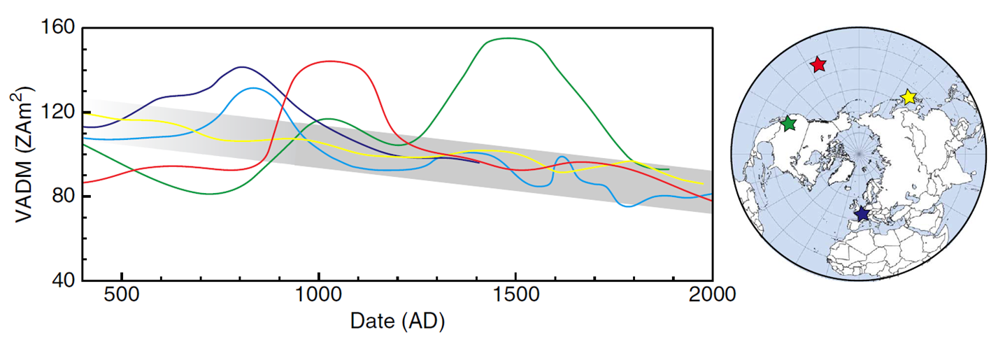
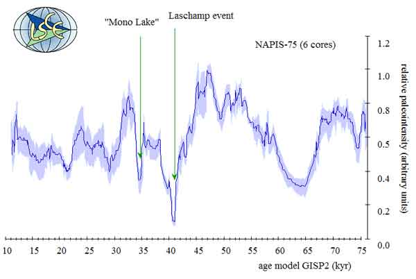
Records of palaeomagnetic strength fluctuations over millions of years have already hinted that the magnetic field displays some “correlation” over hundreds of thousands of years (that is, it may be consistently stronger or weaker on average during one period lasting a few hundreds of thousands of years that during another similarly long period). Our new study reports the first evidence that similar “correlation” may be present in the magnetic field direction as well.

Why is this important? Well, in addition to telling us more about the process that generates the Earth’s magnetic field, it also tells us we need to be careful in making the argument that similar palaeomagnetic directions in adjacent lava flows imply very fast eruption rates (as has been done previously). They may not and, with this requirement for rapid lava extrusion reduced, some of the lethality of the “killer LIPs” could be drawn into question too.

This article was originally posted on the EGU Blog network for Geology Jenga.

Happy New Year to you all!

The past few weeks and months have seen some exciting newsworthy stories regarding the Earth’s magnetic field. I thought I’d highlight a few of them for our first post of the New Year.

Magnetic Interactions 2014

For two days in early January, all of us at the Geomag Lab (well, pretty well all of us) travelled to Cambridge University, to attend the UK conference for the geomagnetism community. This year there was also a strong international presence. I would usually write a blog post on the highlights of the research that was being showcased at the conference; however, the meeting organisers beat me to it! Read about the science behind fundamental, applied rock and mineral magnetism, as well as, how an ancient voyage by naturalist Alexander von Humboldt might help us understand the geomagnetic field prior to the 1800s  in this blog post by Dr. Richard Harrison, of Cambridge University.

Logo courtesy of Richard Harrison.

The Aurora that never was.

Credit: Wikimedia Commons, user: United States Air Force, This image or file is a work of a U.S. Air Force Airman or employee, taken or made as part of that person’s official duties. As a work of the U.S. federal government, the image or file is in the public domain.

On 7^th January, there was a large solar flare with an associated fast traveling Coronal Mass Ejection (CME), which was headed straight for the Earth, and was expected to hit our planet by the 9^th of January. Space weather scientists, the media and people across the UK and Europe were glued to the night skies in hopes of seeing aurora borealis at abnormally southerly latitudes. Perhaps the excitement surrounding the potential to observe these mysterious phenomena was fueled, at least in the UK, by the timely airing of the first episode of the new series of Star Gazing Live, in which the team (made up of Prof. Brian Cox and comedian Dara O’Brien) took on the challenge to capture the northern lights.

Space weather has featured heavily in the UK media in the run up to the Christmas, as the UK government pledged a £4.6 million investment in the forecast of space weather. From early this year, the Met Office will forecast, deliver alerts and warnings to key sectors that might be adversely affected by  solar flares and CMEs.

Despite the hype, the skies did not deliver. A great blog post by Dr Gemma Kelly, at the geomagnetism team of the British Geological Survey, explains the reasons behind why the Northern lights didn’t quite happen!

For more information on solar flares, CMEs and why they are important: have a look at my guest blog post for GeoSphere on the Earth’s protective shield and also the information pages of the British Geological Survey.

We just published a new paper lead-authored by Lennart de Groot at Utrecht University who just recently got his PhD “Cum Laude” (quite a distinction).

The paper is online here and I’ve tried to summarise it below.

The Earth’s magnetic field as seen at Earth’s surface is about 90% explained by a “dipole” – a single north pole opposite a single south pole – the same as a bar magnet. The dipole is not stationary but moves around and fluctuates in intensity over time. Occasionally it collapses altogether and grows back with the opposite polarity – this is called a geomagnetic reversal. The last reversal happened 780,000 years ago but there have been many more recent collapses (“geomagnetic excursions”) that haven’t resulted in reversals.

Two of the authors – Lennart and Mark on the top of Mt Etna in 2008.

The dipole has been weakening steadily (nearly 10%) since the first measurements began in 1840 AD causing some to speculate that we might be heading for a new collapse which would be bad news as magnetic storms might then become more severe. To understand this recent decline, we need to put it in context of magnetic field behaviour before 1840 and for this we have to turn to “accidental” records. The best of these are preserved in baked archaeological materials (e.g. pottery and kiln linings) but these are restricted to locations where complex civilizations existed and this leaves large areas of the globe undocumented.

Records are also preserved in volcanic rocks that have cooled from magma but these are generally much noisier than the archaeological ones because the lavas have less ideal magnetic properties than do pottery. Our study has managed to use a combination of new and old methods to produce a new high quality record from Hawaiian lavas informing us about the behaviour of the field in the sparsely populated Pacific region from around 500 AD to the present.

Combining this new record with other high quality records from archaeological materials recovered from W Europe, Japan, SW USA produces an interesting picture (see figure). As already thought, the recent decline appears to be a continuation of a declining trend going on at least 1,000 year. However, as well as this decline there are also periods of sharply increased intensity in 3 of the records (Hawaii, W Europe, SW USA) but crucially these are at different times in different places (and there is no such peak in Japan). These fluctuations, though large, can’t be explained by the dominant dipole part of the magnetic field as then you would see them everywhere. They must rather be due to the non-dipole field becoming regionally very important in a way that we have not seen since we have been making deliberate records.

Records of the estimated strengh of the main “axial dipole” component of the magnetic field from different locations

The magnetic field is generated by the flow of electrically conducting liquid in the Earth’s outer core and all of these changes reflect the chaotic nature of this flow. In addition to producing records such as these, the challenge lies in producing believable models of core flow to explain the observational data. This might eventually be useful to help predict future magnetic field behaviour.

At the latest magnetic personalities meeting we looked at a paper by Ron Shaar and Lisa Tauxe named ‘Thellier GUI: An integrated tool for analysing palaeointensity data from Thellier type experiments’ published in Geochemistry, Geophysics, Geosystems. I chose this paper as it has direct relevance to the laboratory at Liverpool where we carry out much palaeointensity research.
As with many disciplines in science there is debate over the best methods of analysing data. Ideally there would be a format giving rise to objective results that could be reproducible and correlated between laboratories. Unfortunately this is not the case in the world of palaeointensity study. A plethora of Thellier style palaeointensity methods and analysis make it difficult to correlate across studies. The main issues highlighted by the authors are the subjective nature of manual palaeointensity analyses, that it is very time consuming and that unless the raw data is published the results are not reproducible.

The paper uses two case studies, one from an Iron Age copper slag and another of submarine basaltic glass from a DSDP/ODP cores spanning 160Ma to illustrate how manual interpretation leads to different conclusions dependent on which criteria are selected.

The Thellier GUI integrated tool for palaeointensity analysis is designed to isolate the criteria of most importance during analyses at the specimen and sample stages. It incorporates two new tools, the ‘Auto Interpreter’ and the ‘Thellier Consistency Test’. New statistics include FRAC, a fraction statistic and a new scatter statistic amalgamating all scatter including pTRM and tail checks called SCAT, and finally GAP-MAX an upper limit for the gap between data points in an Arai plot. Sample level palaeointensity values are then calculated using an optimised standard deviation statistic and simple and parametric bootstrap methods.

Snapshot of GUI main screen

We unanimously agree there should be more uniformity in this field and hopefully this tool will go some way towards this. Uniformity of methods and analysis would greatly benefit our models of magnetic field behaviour where correlation of worldwide studies is paramount. We look forward to applying this approach to our own data sets. Work is also underway to integrate the Liverpool Palaeomagnetic Database with the MagIC database to encourage the standardisation of data format and consistency of analyses.

Shaar, R, & Tauxe, L. (2013), ‘Thellier GUI: An integrated tool for analyzing paleointensity data from Thellier-type experiments’, Geochemistry Geophysics Geosystems, 14, 3, pp. 677-692

Last week, Megan and I were away in Oxford taking part in a National Environmental Research Council (NERC) sponsored young entrepreneurs competition. The competition is called, EnvironmentYES! (Think Dragon’s Den!). In the competition, teams of early-career researchers (PhD students and post-dcos) attend a three-day workshop where they are given training and guidance on innovation and how to commercialise research. At the end of the three-day workshop, teams present and pitch their ideas for an imaginary environmental start-up company in competition with each other. The winning teams from each workshop are invited to a final where they compete for a prize of £2500.

Meet the team! Steve, Laura, Megan and Lidong (L-R).

Megan and I are part of a four person team taking part in the competition. One of our fellow PhD students in the school, Steve Hicks, approached us towards the end of the summer, to see if we fancied having a go at the competition. We both agreed to do it as it was an opportunity to learn about the business world, which we knew little about.  Lidong Bie decided to join our team, and so we could get to work! This kick started a few months of preparation for the workshop in Oxford last week.

The first thing we had to do was decide what our product was going to be. We had LOTS of ideas: some quite sensible, whilst others where a little out there. Eventually, we managed to narrow it down to three ideas: using pea straw for the remediation of contaminated land, developing a service to monitor seismicity associated with fracking activities and the monitoring of air quality by measuring magnetic particles on tree leaves. Two of our ideas were based on already published research, which you can read all about here and here.  As it is a business competition, we had to assign ourselves roles within the management of our fictitious company. Steve took on the role of CEO, Lidong became our finance man, Megan is in charge of marketing, whilst I am our research and development officer (i.e, I’m in charge of the science).

Steve approached The University Graduate School, Management School and Technology Transfer Services, all of whom have provided us with lots of help in preparing for the competition. During our first meeting with them, we ‘pitched’ our three ideas (note how I am already slipping into my newly acquired business and commercial vocabulary). When starting a business, as we quickly found out, the idea is important, but not as important as identifying who has a need for the product/service you are offering, i.e. what and who make your market? This was something we thought about a lot when deciding which idea to go with. With the fracking and air quality monitoring ideas we just couldn’t really see who would buy our services/products and so in the end, we settled with remediating contaminated land using pea straw; and so team TERGEO was born.

Our company Logo

Having chosen our idea we had to formulate it into a viable, appealing and realistic business proposition. I got on with really understanding the science behind the idea and explained to the team how the world of environmental consultancy worked (as I worked as a consultant before I started my PhD). Megan worked hard on identifying who are customers and competition would be. Lidong had the arduous task of getting to grips with endless financial spread sheets and costing up both our site works and overall business running costs. Steve coordinated all the work and researched how we could ‘protect our idea’. Intellectual property and how you can protect ideas, products and know how is fascinating and at the same time, extremely complex.

All our hard work culminated last week, when we attended the workshop in Oxford. The first two days were dedicated to learning more about how to set-up your own business, receiving help and support from a wide range of mentors and hearing from people who have actually gone on to set up their own company (some as a result of participating in the competition). The final day of the workshop saw all the teams go up against each other in front of a panel of ‘investors’. We had to deliver 15 minute business presentations, to compete for the judge’s investment in our company. Our team was put into the first stream (of two), and we competed against five other teams. Some of the ideas pitched by other teams were incredibly interesting: tents with built in solar panels, an app that worked out what the most eco-friendly products available in a supermarket are, a chip that monitors your UV exposure, a  pressure driven turbine that generates power from the main water supply and a solar panel with a kick!  Teams fielded questions from the investors really well and people were so enthusiastic about their idea and business!

The judges verdict was announced at 3pm on Friday afternoon, to a room packed full of expectant participants and mentors. Team TERGEO are super excited to announce that we made it through the regional finals and are now on our way to Grand Final in London on 2^nd December! Watch this space!

Acknowledgements

We couldn’t have got as far as we did in the competition without the help of our mentors. So a big thank you to:

Dr. Dale Heywood, Director of Entrepreneurship studies at the University of Liverpool

Dr. Richard Hinchcliffe, Head of Postgraduate Development at the University of Liverpool.

Dr.Lisa Ahmead, Partnerships and Innovation, Business Gateway, University of Liverpool

Andrew Bowen, ISIS Innovation

Luca Guerzoni, Esperimenta

Becky Herbert, Alan Garmonsway, Emma Faldon, The Pirbright Institute

Bevan McWilliam, RVC Enterprise

SWARM is a long awaited ESA satelite mission to measure the geomagnetic field using magnetometers deployed on three separate but identical satelites.

They have a nice blog showing the build-up to the launch and with links to the mission details:

http://blogs.esa.int/eolaunches/

It has been a long time coming…

The International Association of Geomagnetism and Aeronomy meets every 4 years in different international locations.  The most recent of these was in Merida, Mexico and 4 members of the Liverpool geomagnetism laboratory went along to present their most recent findings, hear about current developments in the field and catch up with other scientists interested in palaeomagnetism and geomagnetism based around the world.   It was a fascinating experience for me as it was my first international conference as well as being the biggest I have attended so far!  There were between 500 and 550 delegates at the meeting including Neil Sutie, Andreas Nilsson, John Shaw and myself from the University of Liverpool.  We tended to attend the same sessions and heard a range of talks from environmental magnetic proxies to magnetic anisotropy to tectonic plate reconstructions to archaeomagnetism.

The most interesting talk for me personally was given by Elina Aidona from the Aristole University of Thessaloniki, Greece who had conducted a study on archaeological ovens and found that the errors on the archaeomagnetically assigned age was lower than the errors on the thermoluminescence dates.  This is highly unusual and was a very interesting case study.

Andreas and I visiting the local Mayan site of Uxmal

In addition to attending the most relevant sessions it was nice to hear about how others view and study the magnetic field.  I particularly enjoyed a talk by Ciaran Beggan of the British Geological Survey detailing the potential threat posed to the national grid from magnetic storms.  It was comforting to hear that as the UK’s grid is highly interconnected, in the event of a magnetic storm, the excess electricity generated by the interaction of the Sun’s magnetic field with the Earth’s magnetic field and transported along the grid, should dissipate relatively quickly.  For more detail about this see here: http://nora.nerc.ac.uk/502627/

In the most recent Magnetic Personalities meeting we looked at a paper published in Quaternary Science Reviews in 2005 entitled “Geomagnetic Field intensity during the last 60,000 years based on ¹⁰Be and ³⁶Cl from the Summit ice cores and ¹⁴C” by the authors Raimund Muscheler et al. I chose this paper as I thought it would be interesting to discuss a paper that approaches the problem of geomagnetic field reconstruction in a very different way.

The authors reconstructed past changes in the geomagnetic field intensity based on ¹⁰Be, ³⁶Cl and ¹⁴C records under the assumption that radionuclide records are mainly influenced by changes in their production rates.  Most reconstructions of the geomagnetic field intensity are based on the natural remanent magnetisation acquired by ceramics, volcanic rocks or lacustrine and marine sediments.   

Cosmogenic radionuclides (e.g. ¹⁰Be, ³⁶Cl and ¹⁴C) are produced in the Earth’s atmosphere by the interaction of galactic cosmic rays with the atoms of the atmosphere.  The connection between cosmogenic radionuclide production and the Earth’s magnetic field is as follows: the higher the geomagnetic field intensity, the stronger the deflection of the primary cosmic ray particles that consist mainly of protons and α-particles.  As a consequence, less cosmogenic radionuclides are produced during periods of high geomagnetic field intensity and more are produced in low geomagnetic field intensities.  There are a number of other factors that could influence cosmogenic radionuclide which the authors detail in the paper.

By combining the data from the GRIP and GISP2 ice cores from Central Greenland, it is possible to obtain a continuous record of the deposition of cosmogenic radionuclides in Greenland for the last 60,000 years.  As a group we discussed the results and generally were more convinced by the trends seen in the ¹⁰Be results than the other radionuclides.  We also discussed how well the Laschamp geomagnetic excursion showed up in the data, an event which was first reported in 1969 by Bonhommet and Zähringer.

All in all, it was a very interesting paper to study and its always good to sit in the sunshine and discuss a paper that tackles a problem in an interesting way!

The latest in our paper discussions took us away from our usual  territory- and out to Saturn. Cao et al’s paper Saturn’s high degree magnetic moments: Evidence for a unique planetary dynamo looks at modelling the magnetic field of Saturn, which is very different to the field of the Earth. Parts of the magnetic field have been measured by Pioneer 11, and both Voyager missions, and more recently, Saturn has been visited by the Cassini mission, which also recorded magnetic data, and essentially confirmed what was already known. Analysis of the data from Pioneer and Voyager(s) and modelling of low spherical harmonic degrees (g⁰₁, g⁰₂ and g⁰₃) show Saturn’s field to be highly axisymmetric (i.e. symmetrical around the spin axis, with little difference as you move along the equator but poles of opposite sign) and also much weaker than the field of the Earth, being around 30,000nT at the surface, compared to 50,000nT here. The field axis is the same as the rotational axis, to within 0.06^o. There has also been very little change in the field measured between the Voyager missions and Cassini’s arrival. The magnetic moments of the lower spherical harmonic degrees having being well modelled with the available data, in this paper the authors try to model higher degrees, g⁰₄ and g⁰₅ with the new data from Cassini.

Cassini probe approaching Saturn

The results they find agree with what was previously found – that Saturn’s field is highly axisymmetric, with most of the magnetic flux confined to polar regions, and higher degrees of the field are relatively small contributions to the overall measured field – hence not being seen on some more distant orbits of the satellite. They also suggest a similarity to certain types of dynamo models – such as spherical Couette dynamos, where the dynamo is driven by differential rotation between outer and inner layers of a shell. This is a very different type of dynamo to the Earth, with its convection driven dynamo – and indeed may not even be physically possible for Saturn! In this case, the different rotations could be due to a transition in the phase of helium (such as the gaseous atmosphere ‘raining’ liquid helium at pressure), a metallic layer, or the solid core of the planet. This was certainly the part of the paper that provoked most discussion amongst us – and several sci-fi type visualisations of what helium rain might look like!

Cao, H, Russell, C, Wicht, J, Christensen, U, and Dougherty, M.  Icarus 221, 2012, 388–394: Saturn’s high degree magnetic moments: Evidence for a unique planetary dynamo.

Today’s post was guest written by Kelly Barker. Kelly is a PhD student in the geomagnetism research group at the Department of Earth, Ocean and Ecological Sciences at the Univeristy of Liverpool. Her research project is entitled: Improved application of remote referencing data in aeromagnetic processing: insights and applications from global geomagnetic modelling.

I am afraid this post is a little delayed. The paper we discussed at the end of June was: Alteration and self-reversal in oceanic basalts, Doubrovine & Tarduno, 2006. A companion paper, well worth a look at is: Self-Reversal magentization carried by titanomaghemite in oceanic basalts, Doubrovine & Tarduno (2004).

I chose this paper because of some intriguing results I’ve had working on my Archean aged samples. I was keen to hear what the lab had to say about the paper above, but also about my results and self-reversals in general, as they are pretty controversial due to being quite poorly understood.

It has been suggested, since the late 1950s, that given the right conditions, some oceanic basalts can carry a self-reversed chemical remanent magnetisation (CRM). Research by Verhoogen (1956) suggested that self-reversals could occur in titanomagnetites by ionic reordering during low-temperature oxidation.  Oceanic basalts are good candidates because seafloor weathering is characterised by low-temperature oxidation of titanomagnetites as show by Bleil & Petersen, 1983, amongst others. However, it was not until the research published in Doubrovine & Tarduno, 2004, that a clear example of this process was identified and so, little research into self-reversals was conducted during the 1990s.

In oceanic basalts, oxidation occurs by the removal of iron due to interaction with sea water or sea water bearing fluids. Self-reversals occur at a critical degree of oxidation when it is possible for cation vacancies created at tetrahedral sites (A magnetic sublattice) to migrate into the octahedral sublattice, via diffusion. This process is known as Ionic Reordering . It allows single domain grains (and perhaps also pseudosingle domain grains) that carry a CRM by titanomagnetite to transform into an antipodal CRM. I recommend you take a look at the two papers if you want to understand this process more fully, they’ve got some good formulas which might help!

Verhoogen (1956) reported a large range of titmanomagnetite compositions were this process might be possible (light grey area in theTiO₂-FeO-Fe₂O₃ diagram), but O’Reilly & Banerjee (1966) showed that Verhoogen’s (1956) cation distribution was unrealistic and indicated that self-reversals were only possible in titanomaghemite, (dark grey area in theTiO₂-FeO-Fe₂O₃ diagram). In addition, work by Schult (1968, 1971) shows that ionic reordering should produce N or Q-type thermomagentic behaviour.

The work by Doubrovine & Tarduno (2004,2006) suggests that the compositional field in which true self-reversals can occur, as proposed by O’Reilly & Banerjee (1966) is too broad and that the range is in fact, much more restricted than previously though. The work presented in the paper suggests that the very high oxidation states and high Ti contents are required to produce a true self-reversals negates the possibility of it being a common occurrence in oceanic basalts. The authors suggest that self-reversal is indicative of unusual ocean floor conditions such as extreme fluid flow and iron removal.

Selected References

Bleil, U., and N.Peteresen (1983), Variations in magnetization intensity and low-temperature titanomagnetite oxidation of ocean floor basalts, Nature, 301, 384-388.

O’Reilly, W,. and S.K. Banerjee (1966), Oxidation of titanomagnetites and self-reversal, Nature, 211 (5044), 26-28

Schult, A. (1968), Self-reversal of magnetization and chemical composition of titanomagnetites in basalts, Earth Planet Sci. Lett., 4, 57-63.

Verhoogen,J. (1956), Ionic reordering and self-reversal magnetization in impure magnetities. J.Geophys. Res., 61(2), 201-209